Typography

Text can be bold, italic, strikethrough, or inline code.

 *italic*
 **bold**
 ~~strikethrough~~
 `inline code`
[link](https://example.com)

Code Blocks

R Code

ggplot(gapminder) +
  aes(x = gdpPercap, y = lifeExp, size = pop, color = country) +
  geom_point() +
  facet_wrap(~year)

Tables

knitr::kable(head(mtcars), format = 'html')

DT::datatable(head(mtcars), fillContainer = FALSE, options = list(pageLength = 4))

The markdown is:

 * Item foo
 * Item bar

And a nested list:

• level 1 item
  • level 2 item
  • level 2 item
  • level 3 item
  • level 3 item
• level 1 item
  • level 2 item
  • level 2 item
  • level 2 item
• level 1 item
  • level 2 item
  • level 2 item
• level 1 item

Nesting an ol in ul in an ol

• level 1 item (ul)
  1. level 2 item (ol)
  2. level 2 item (ol)
  • level 3 item (ul)
  • level 3 item (ul)
• level 1 item (ul)
  1. level 2 item (ol)
  2. level 2 item (ol)
  • level 3 item (ul)
  • level 3 item (ul)
  1. level 4 item (ol)
  2. level 4 item (ol)
  • level 3 item (ul)
  • level 3 item (ul)
• level 1 item (ul)

Images

Data Visualization

• ggplot is great for fast exploratory plots.
• It has great tools for creating plots for communicating your results.
• In this scenario, the emphasis should be on the story you are trying to tell.

Themes

• Branding example from the BBC

Default theme

• Is called theme_grey()

ggplot(diff_df, aes(x = pts_diff, y = win_pct)) +
  geom_point() + 
  theme_grey()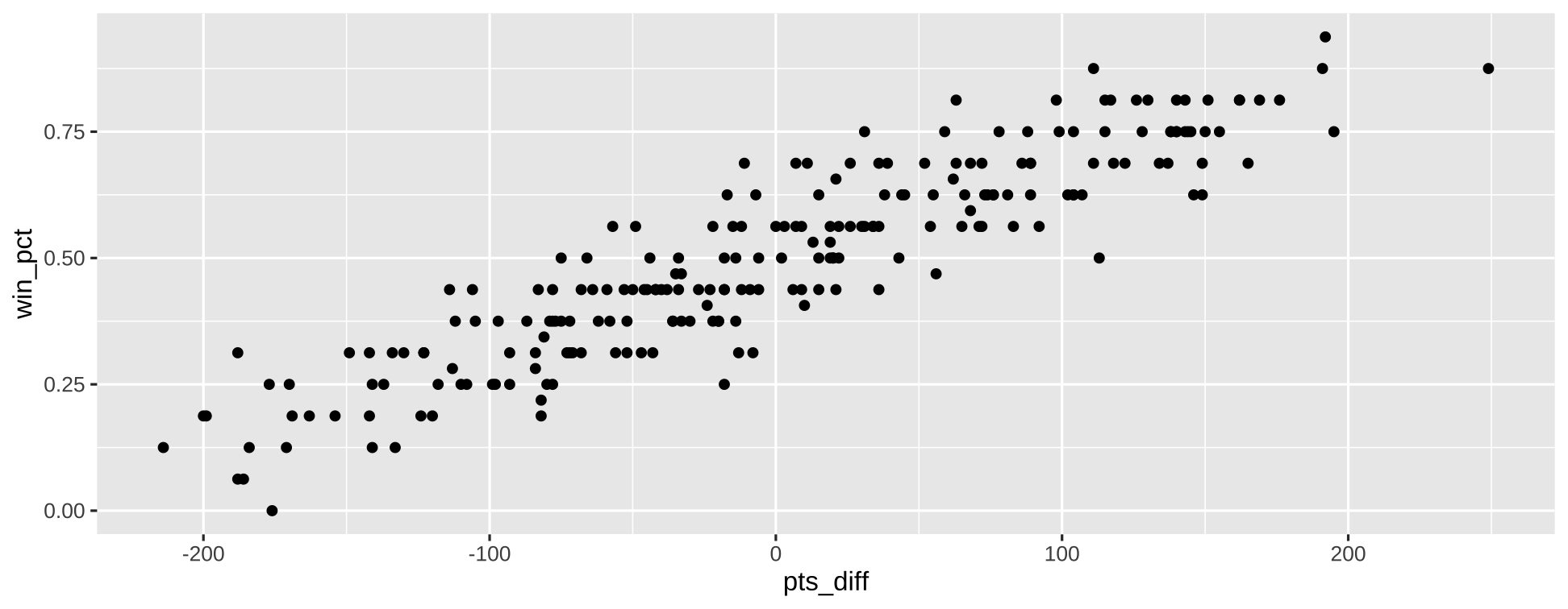

• Grey panel background
• white grid lines

GGthemes

• package with some well known themes:
  • theme_fivethirtyeight()
  • theme_economist()

Theme elements

• theme elements can be lines, text, etc.
• To specify an option, you use the corresponding element.

Centering titles and subtitles

• When styling text, use element_text.

theme(
  plot.title=element_text(hjust=.5)
)

Grids

• When styling lines, use element_line

theme(
  panel.grid.major=element_line(color="red")
)

Labels

plot <- nfl_stand %>% 
  mutate(
    color = case_when(
      season < 2020 & seed <= 6 ~ "blue",
      season == 2020 & seed <= 7 ~ "blue",
      TRUE ~  "red"
    )
  ) %>% 
  ggplot(aes(x = as.numeric(pts_diff), y = win_pct)) +
  geom_vline(xintercept = 0, size = 0.75, color = "#737373") +
  geom_point(
    aes(color = color),
    size = 3, alpha = 0.8
    ) +
  scale_color_identity() +
  labs(x = "Points Differential", y = "Win Percent",
       title = "Playoff teams typically have a positive point differential",
       subtitle = "Data through week 15 of the 2020 NFL Season",
       caption = "Plot: @thomas_mock | Data: ESPN")

plot

Scales

plt_scales <- nfl_stand %>% 
  mutate(
    color = case_when(
      season < 2020 & seed <= 6 ~ "blue",
      season == 2020 & seed <= 7 ~ "blue",
      TRUE ~  "red"
    )
  ) %>% 
  ggplot(aes(x = as.numeric(pts_diff), y = win_pct)) +
  geom_vline(xintercept = 0, size = 0.75, color = "#737373") +
  geom_point(aes(color=color)) + 
  scale_color_identity()+
  scale_y_continuous(
    labels = scales::percent_format(accuracy = 1),
    breaks = seq(.0, 1, by = .10)
    ) +
  scale_x_continuous(
    breaks = seq(-200, 250, by = 50)
  ) +
  labs(x = "Points Differential", y = "Win Percent",
       title = "Playoff teams typically have a positive point differential",
       subtitle = "Data through week 15 of the 2020 NFL Season",
       caption = "Plot: @thomas_mock | Data: ESPN")

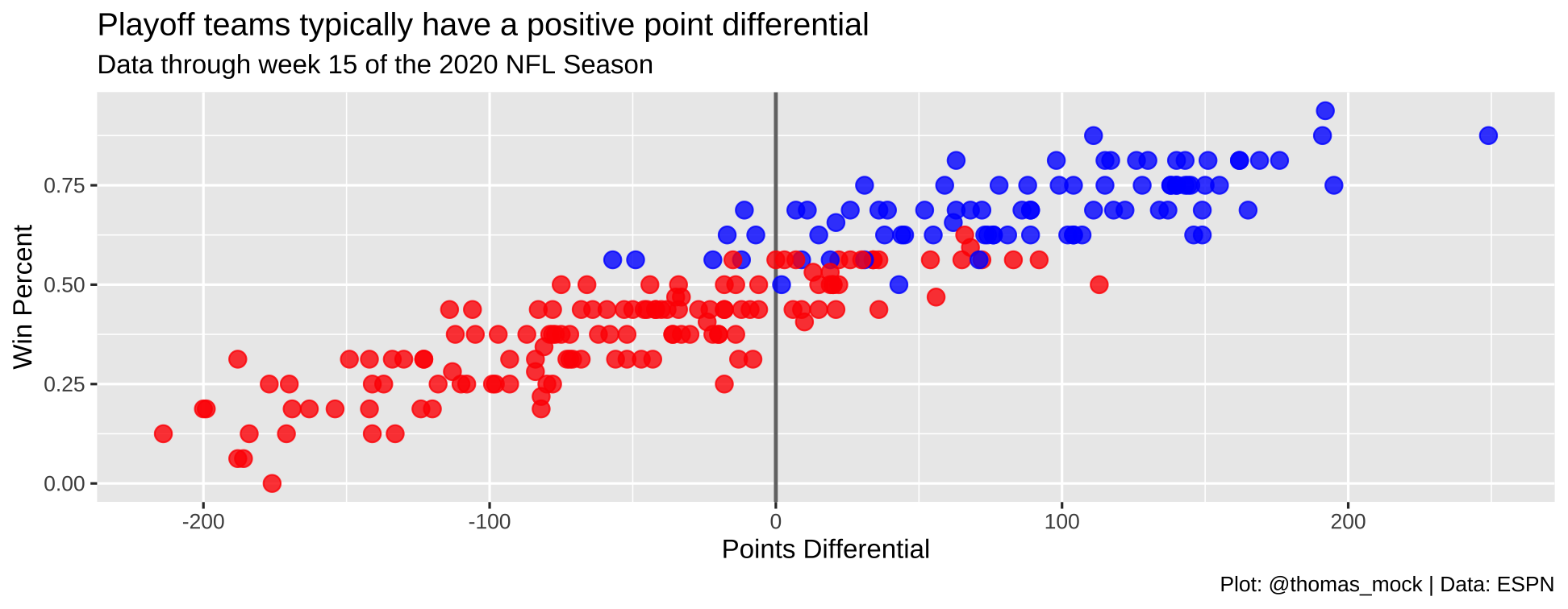
plt_scales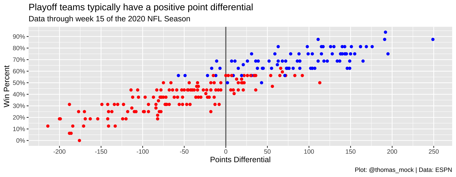

Experiment with themes

plot + ggthemes::theme_economist()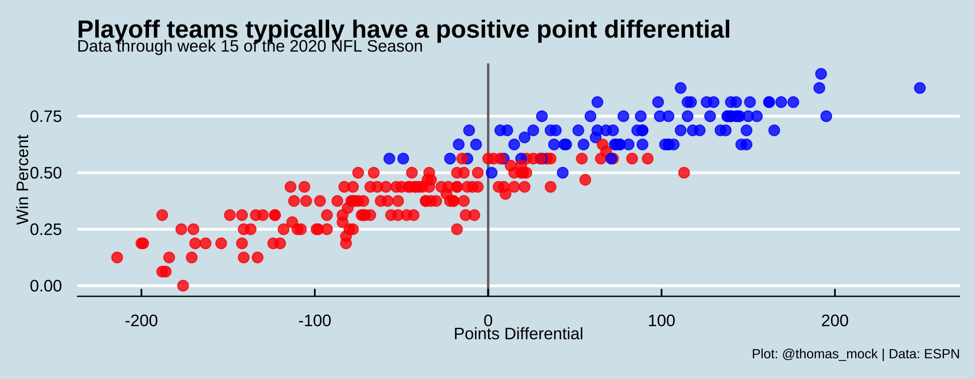

Final plot

library(ggtext)
playoff_label_scatter <- tibble(
  pts_diff = c(25,-125), y = c(0.3, 0.8), 
  label = c("Missed<br>Playoffs", "Made<br>Playoffs"),
  color = c("#D50A0A", "#013369")
)
playoff_diff_plot <- nfl_stand %>% 
  mutate(
    pts_diff=as.numeric(pts_diff),
    color = case_when(
      season < 2020 & seed <= 6 ~ "#013369",
      season == 2020 & seed <= 7 ~ "#013369",
      TRUE ~  "#D50A0A"
    )
  ) %>% 
  ggplot(aes(x = pts_diff, y = win_pct)) +
  geom_vline(xintercept = 0, size = 0.75, color = "#737373") +
  geom_hline(yintercept = 0, size = 0.75, color = "#737373") +
  geom_point(
    aes(color = color),
    size = 3, alpha = 0.8
    ) +
  # ggtext::geom_richtext(
  #   data = playoff_label_scatter,
  #   aes(x = pts_diff, y = y, label = label, color = color),
  #   fill = "#f0f0f0", label.color = NA, # remove background and outline
  #   label.padding = grid::unit(rep(0, 4), "pt"), # remove padding
  #   family = "Chivo", hjust = 0.1, fontface = "bold",
  #   size = 8
  # ) +
  scale_color_identity() +
  labs(x = "Points Differential", y = "Win Percent",
       title = "Playoff teams typically have a positive point differential",
       subtitle = "Data through week 15 of the 2020 NFL Season",
       caption = str_to_upper("Plot: @thomas_mock | Data: ESPN")) +
  scale_y_continuous(
    labels = scales::percent_format(accuracy = 1),
    breaks = seq(.0, 1, by = .10)
    ) +
  scale_x_continuous(
    breaks = seq(-200, 250, by = 50)
  ) + 
  theme(plot.subtitle=element_text(hjust=.5))